What follows is a brief description of the approximation used to calculate the evolution of the wave function. Formulas of the evolution operator are provided.

Lattice

The wave function is defined using the coordinate representation ( \(\psi(x,y) = \langle x,y|\psi\rangle\)). The coordinates parametrize a 'physical space'. These can be cartesian coordinates for 1D or 2D space, or cylindrical coordinates in 1D (only radial coordinate) or 2D (radial and axial coordinates). For computational reasons, the 'physical space' is finite, and each coordinate takes values on the intervals \(x \in [-L_x/2,L_x/2]\), \(y \in [-L_y/2,L_y/2]\) (cartesian coordinates) and \(r \in [0,L_r]\), \(z \in [-L_z/2,L_z/2]\) (cylindrical coordinates). The wave function is discretize in a lattice: for cartesian coordinates \(\psi(x,y)\) with \(x\) and \(y\) integer numbers: \(x = 0, 1, \ldots N_x-1\), \(y = 0, 1, \ldots N_y-1\), and similarly for the cylindrical coordinates: \(\psi(r,z)\) with \(r = 0, 1, \ldots N_r-1\), \(z = 0, 1, \ldots N_z-1\).

MPI structure

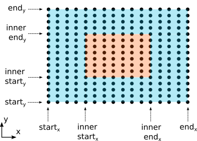
The evolution of the wave function can be distributed among independent processes, using the MPI framework. The lattice is divided in a number of smaller lattices, called tiles, equal to the number of available processes. Each process evolves the part of the wave function defined over the tile it has. In particular, each tile possesses points shared between neighbouring processes (cyan region) and points that are not shared (orange region). The former are needed to ensure stability of the evolution of the wave function inside the orange region. The integer numbers 'start-x', 'inner-start-x', ecc. define the size of the regions and they are calculated by the function 'calculate-borders'. Each point of the tile is mapped to a point of the physical space by the function 'map-lattice-to-coordinate-space', which is described in the next section.

Example of a two-dimensional tile of a single process. Points in the cyan region (halo) are shared among neighbouring processes to ensure stability of the evolution of the wave function inside the orange region.

Mapping coordinates of the lattice to the physical space

A point \((i,j)\) of the tile is mapped to a point in the physical space, where the wave function is defined, as

\begin{equation} \begin{aligned} x &= \Delta x \left(i - \frac{N_x-1}{2} + st_x\right) \\ y &= \Delta y \left(j - \frac{N_y-1}{2} + st_y\right) \end{aligned} \end{equation}

for cartesian coordinates, where \(\Delta x = L_x / N_x\), \(\Delta y = L_y / N_y\) and \(st_x\) and \(st_y\) are respectively start-x and start-y. On the other hand, cylindrical coordinates are mapped with a different map. In this case when the user define \(N_r\) points in the lattice along the radial coordinate, another point is added so that it has a negative radial value (this point is needed to ensure the stability of the evolution). Then, the map is

\begin{equation} \begin{aligned} r &= \Delta r \left(i - \frac{1}{2} + st_r\right) \\ z &= \Delta z \left(j - \frac{N_z-1}{2} + st_z\right) \end{aligned} \end{equation}

where \(\Delta_r = L_r / (N_r + \frac{1}{2})\) and \(\Delta z = L_z / N_z\).

Evolution operator

The evolution operator is calculated using the Trotter-Suzuki approximation. Given an Hamiltonian as a sum of hermitian operators, for instance \(H = H_1 + H_2 + H_3\), the evolution is approximated as

\begin{equation} e^{-i\Delta tH} = e^{-i\frac{\Delta t}{2} H_1} e^{-i\frac{\Delta t}{2} H_2} e^{-i\frac{\Delta t}{2} H_3} e^{-i\frac{\Delta t}{2} H_3} e^{-i\frac{\Delta t}{2} H_2} e^{-i\frac{\Delta t}{2} H_1}. \end{equation}

Since the wavefunction is discretized in the space coordinate representation, to avoid Fourier transformation, the derivatives are approximated using finite differences.

Kinetic operators

In cartesian coordinates, the kinetic term is \(K = -\frac{1}{2m} \left( \partial_x^2 + \partial_y^2 \right)\). The discrete form of the second derivative is

\begin{equation} \partial_x^2 \psi(x) = \frac{\psi(x + \Delta x) - 2 \psi(x) + \psi(x - \Delta x)}{\Delta x^2} \end{equation}

It is useful to express the above equation in a matrix form. The wave function can be vectorized as it is discrete, hence the partial derivative is the matrix

\begin{equation} \begin{aligned} \frac{1}{\Delta x^2} \left(\begin{array}{ccc} -2 & 1 & 0 \\ 1 & -2 & 1 \\ 0 & 1 & -2 \end{array} \right) =& \frac{1}{\Delta x^2} \left(\begin{array}{ccc} 0 & 1 & 0 \\ 1 & 0 & 0 \\ 0 & 0 & 0 \end{array} \right) + \frac{1}{\Delta x^2} \left(\begin{array}{ccc} 0 & 0 & 0 \\ 0 & 0 & 1 \\ 0 & 1 & 0 \end{array} \right)\\ &- \frac{2}{\Delta x^2} \left(\begin{array}{ccc} 1 & 0 & 0 \\ 0 & 1 & 0 \\ 0 & 0 & 1 \end{array} \right). \end{aligned} \end{equation}

On the right-hand side of the above equation the last matrix is the identity and in the approximation of Trotter-Suzuki it gives only a global shift of the wave function, which can be ignored. The other two matrices are in the diagonal block form and can be easily exponentiated. Indeed, for the real time evolution:

\begin{equation} \exp\left[i\frac{\Delta t}{4m \Delta x^2} \left(\begin{array}{cc} 0 & 1 \\ 1 & 0 \end{array} \right)\right] = \left(\begin{array}{cc} \cos\beta & i\sin\beta \\ i\sin\beta & \cos\beta \end{array} \right). \end{equation}

While, for imaginary time evolution:

\begin{equation} \exp\left[\frac{\Delta t}{4m \Delta x^2} \left(\begin{array}{cc} 0 & 1 \\ 1 & 0 \end{array} \right)\right] = \left(\begin{array}{cc} \cosh\beta & \sinh\beta \\ \sinh\beta & \cosh\beta \end{array} \right), \end{equation}

with \(\beta = \frac{\Delta t}{4m \Delta x^2}\).

In cylindrical coordinates, the kinetic operator has an additional term, \(K = -\frac{1}{2m} \left( \partial_r^2 + \frac{1}{r} \partial_r+ \partial_z^2 \right)\). The first derivative is discretized as

\begin{equation} \frac{1}{r}\partial_r \psi(r) = \frac{\psi(r + \Delta r) - \psi(r - \Delta r)}{2 r \Delta r}, \end{equation}

and in matrix form

\begin{equation} \frac{1}{2 \Delta r} \left(\begin{array}{ccc} 0 & \frac{1}{r_0} & 0 \\ -\frac{1}{r_1} & 0 & \frac{1}{r_1} \\ 0 & -\frac{1}{r_2} & 0 \end{array} \right) = \frac{1}{2 \Delta r} \left(\begin{array}{ccc} 0 & \frac{1}{r_0} & 0 \\ -\frac{1}{r_1} & 0 & 0 \\ 0 & 0 & 0 \end{array} \right) + \frac{1}{2 \Delta r} \left(\begin{array}{ccc} 0 & 0 & 0 \\ 0 & 0 & \frac{1}{r_1} \\ 0 & -\frac{1}{r_2} & 0 \end{array} \right). \end{equation}

The exponentiation of a block is, for real-time evolution:

\begin{equation} \exp\left[i\frac{\Delta t}{8m \Delta r} \left(\begin{array}{cc} 0 & \frac{1}{r_1} \\ -\frac{1}{r_2} & 0 \end{array} \right)\right] = \left(\begin{array}{cc} \cosh\beta & i\alpha\sinh\beta \\ -i\frac{1}{\alpha}\sinh\beta & \cosh\beta \end{array} \right). \end{equation}

While, for imaginary time evolution:

\begin{equation} \exp\left[\frac{\Delta t}{8m \Delta r} \left(\begin{array}{cc} 0 & \frac{1}{r_1} \\ -\frac{1}{r_2} & 0 \end{array} \right)\right] = \left(\begin{array}{cc} \cos\beta & \alpha\sin\beta \\ -\frac{1}{\alpha}\sin\beta & \cos\beta \end{array} \right). \end{equation}

with \(\beta = \frac{\Delta t}{8m \Delta r \sqrt{r_1r_2}}\), \(\alpha = \sqrt{\frac{r_2}{r_1}}\) and \(r_1, r_2 > 0\). However, the block matrix that contains \(1/r_0\) has a different exponentiation, since \(r_0 < 0 \).

In particular \(r_0 = - r_1\) and for the real-time evolution, the block is of the form

\begin{equation} \exp\left[i\frac{\Delta t}{8m r_1\Delta r} \left(\begin{array}{cc} 0 & -1 \\ -1 & 0 \end{array} \right)\right] = \left(\begin{array}{cc} \cos\beta & i\sin\beta \\ i\sin\beta & \cos\beta \end{array} \right) \end{equation}

for imaginary-time evolution

\begin{equation} \exp\left[\frac{\Delta t}{8m r_1\Delta r} \left(\begin{array}{cc} 0 & -1 \\ -1 & 0 \end{array} \right)\right] = \left(\begin{array}{cc} \cosh\beta & \sinh\beta \\ \sinh\beta & \cosh\beta \end{array} \right) \end{equation}

with \(\beta = -\frac{\Delta t}{8m r_1 \Delta r}\).

External potential

An external potential dependent on the coordinate space is trivial to calculate. For the discretization that we use, such external potential is approximated by a diagonal matrix. For real time evolution

\begin{equation} \begin{aligned} \exp[-i\Delta t V] &= \exp\left[-i\Delta t \left(\begin{array}{ccc} V(x_0,y_0) & 0 & 0 \\ 0 & V(x_1,y_0) & 0 \\ 0 & 0 & V(x_2,y_0) \end{array} \right)\right] \\ &= \left(\begin{array}{ccc} e^{-i\Delta t V(x_0,y_0)} & 0 & 0 \\ 0 & e^{-i\Delta t V(x_1,y_0)} & 0 \\ 0 & 0 & e^{-i\Delta t V(x_2,y_0)} \end{array} \right) \end{aligned} \end{equation}

and for imaginary time evolution

\begin{equation} \begin{aligned} \exp[-\Delta t V] &= \exp\left[-\Delta t \left(\begin{array}{ccc} V(x_0,y_0) & 0 & 0 \\ 0 & V(x_1,y_0) & 0 \\ 0 & 0 & V(x_2,y_0) \end{array} \right)\right] \\ &= \left(\begin{array}{ccc} e^{-\Delta t V(x_0,y_0)} & 0 & 0 \\ 0 & e^{-\Delta t V(x_1,y_0)} & 0 \\ 0 & 0 & e^{-\Delta t V(x_2,y_0)} \end{array} \right) \end{aligned} \end{equation}

Self interaction term

The self interaction term of the wave function, \(g|\psi(x,y)|^2\), depends on the coordinate space, hence its discrete form is a diagonal matrix, as in the case of the external potential. In addition, the Lee-Huang-Yang term, \(g_{LHY}|\psi(x,y)|^3\), is implemented in the same way.

Angular momentum

For cartesian coordinates the Hamiltonian containing the angular momentum operator is

\begin{equation} -i \omega\left( x\partial_y - y\partial_x \right). \end{equation}

For the trotter-suzuki approximation, the exponentiation is done separately for the two terms:

First term, real-time evolution, \(\beta = \frac{\Delta t \omega x}{2\Delta y}\)

\begin{equation} \exp[-\Delta t \omega x\partial_y] = \exp\left[-\beta \left(\begin{array}{cc} 0 & 1 \\ -1 & 0 \end{array} \right)\right] = \left(\begin{array}{cc} \cos\beta & -\sin\beta \\ \sin\beta & \cos\beta \end{array} \right) \end{equation}
First term, imaginary-time evolution, \(\beta = \frac{\Delta t \omega x}{2\Delta y}\)
\begin{equation} \exp[i\Delta t \omega x\partial_y] = \exp\left[-\beta \left(\begin{array}{cc} 0 & 1 \\ -1 & 0 \end{array} \right)\right] = \left(\begin{array}{cc} \cosh\beta & i\sinh\beta \\ -i\sinh\beta & \cosh\beta \end{array} \right) \end{equation}
Second term, real-time evolution, \(\beta = \frac{\Delta t \omega y}{2\Delta x}\)
\begin{equation} \exp[\Delta t \omega y\partial_x] = \exp\left[-\beta \left(\begin{array}{cc} 0 & 1 \\ -1 & 0 \end{array} \right)\right] = \left(\begin{array}{cc} \cos\beta & \sin\beta \\ -\sin\beta & \cos\beta \end{array} \right) \end{equation}
Second term, imaginary-time evolution, \(\beta = \frac{\Delta t \omega y}{2\Delta x}\)
\begin{equation} \exp[-i\Delta t \omega y\partial_x] = \exp\left[-\beta \left(\begin{array}{cc} 0 & 1 \\ -1 & 0 \end{array} \right)\right] = \left(\begin{array}{cc} \cosh\beta & -i\sinh\beta \\ i\sinh\beta & \cosh\beta \end{array} \right) \end{equation}